One sample proportion tests and confidence intervals are covered in Section 6.1 of the Lock 5 textbook.
In the last lesson you were introduced to the general concept of the Central Limit Theorem. The Central Limit Theorem states that if the sample size is sufficiently large then the sampling distribution will be approximately normally distributed for many frequently tested statistics, such as those that we have been working with in this course. When discussion proportions, we sometimes refer to this as the Rule of Sample Proportions. According to the Rule of Sample Proportions, if \(np\geq 10\) and \(n(1-p) \geq 10\) then the sampling distributing will be approximately normal. When constructing a confidence interval \(p\) is not known but may be approximated using \(\widehat p\). When conducting a hypothesis test, we check this assumption using the hypothesized proportion (i.e., the proportion in the null hypothesis).
If assumptions are met, the sampling distribution will have a standard error equal to \(\sqrt>\).
This method of constructing a sampling distribution is known as the normal approximation method.
If the assumptions for the normal approximation method are not met (i.e., if \(np\) or \(n(1-p)\) is not at least 10), then the sampling distribution may be approximated using a binomial distribution. This is known as the exact method. This course does not cover the exact method in detail, but you will see how these tests may be performed using Minitab.
On the following pages you will see how a confidence interval for a population proportion can be constructed by hand using the normal approximation method. Using Minitab, you will learn how to construct a confidence interval for a proportion using the normal approximation method or the exact method. When given the option, it is recommended that you use Minitab as opposed to performing calculations by hand.
For the following procedures, the assumption is that both \(np \geq 10\) and \(n(1-p) \geq 10\). When we're constructing confidence intervals \(p\) is typically unknown, in which case we use \(\widehat
\) as an estimate of \(p\).
Note that \(n \widehat p\) is the number of successes in the sample and \(n(1- \widehat p)\) is the number of failures in the sample.
This means that our sample needs to have at least 10 "successes" and at least 10 "failures" in order to construct a confidence interval using the normal approximation method.
Below is the general form of a confidence interval.
General Form of Confidence Interval \(sample\ statistic\pm\underbrace_>\)The sample statistic here is the sample proportion, \(\widehat p\). When using the normal approximation method the multiplier is taken from the standard normal distribution (i.e., z distribution). And, the standard error is computed using \(\widehat p\) as an estimate of \(p\): \(\sqrt <\frac<\hat
(1-\hat
)>>\). This leaves us with the following formula to construct a confidence interval for a population proportion:
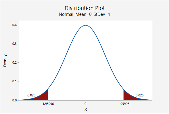
The value of the \(z^*\) multiplier depends on the level of confidence. The multiplier for the confidence interval for a population proportion can be found using the standard normal distribution [i.e., z distribution, N(0,1)]. The most commonly used level of confidence is 95%. As shown on the probability distribution plot below, the multiplier associated with a 95% confidence interval is 1.960, often rounded to 2 (recall the Empirical Rule and 95% Rule).
Below is a table of frequently used \(z^*\) multipliers.
| Confidence Level | \(z^*\) Multiplier |
|---|---|
| 90% | 1.645 |
| 95% | 1.960, often rounded to 2 |
| 98% | 2.327 |
| 99% | 2.576 |
The value of the multiplier increases as the confidence level increases. This leads to wider intervals for higher confidence levels. We are more confident of catching the population value when we use a wider interval.